How EPSS Works
Data Sources
Each daily vulnerability record is built from approximately 2,850 features drawn from several distinct source categories. The features span from signals that exist the day a vulnerability is disclosed to signals that only emerge weeks or months later as the security community and attacker ecosystem respond.
Exploit code and offensive tooling. The presence of public exploit code is one of the strongest signals in the model. But rather than simply asking if exploit code exists or not, EPSS asks what kind of exploit code, published where, and how widely has it been adopted? There is a difference between carefully tested exploit code that is operationalized in an exploit framework and a proof-of-concept pasted to a personal blog. Beyond exploit code, EPSS tracks whether a vulnerability has been incorporated into various operational attacker tooling like Nuclei templates and Shodan. Some of the signals in the category may correlate with exploitation because they follow attacker attention. Others correlate because they create it.
Chatter. EPSS monitors which security-relevant domains reference a vulnerability and how recently that activity occurred. The sources span a wide range: security vendors whose coverage reflects telemetry from deployed detection products, internet monitoring platforms that track active scanning and exploitation traffic, coordinated disclosure programs, informal channels where exploit code surfaces before reaching formal repositories, community aggregators and social platforms, and OS and distribution advisories. Each source domain is treated as a distinct feature, and each carries different signal properties. Some lead exploitation, some lag it. The recency signals capture how recently that discussion has occurred, using time-bounded reference counts across those sources. Together, where a vulnerability is discussed and when reflects the security community's current attention, which correlates with attacker attention.
Vulnerability characteristics. EPSS uses the individual metrics from CVSS as features, covering both the exploitability metrics (attack vector, attack complexity, privileges required, user interaction) and the impact metrics (confidentiality impact, integrity impact, availability impact). By ignoring the score and focusing on the underlying metrics, the model discovers what weight each carries rather than accepting the aggregation formula CVSS applies. Impact metrics are included because vulnerabilities enabling high-confidentiality or code-execution outcomes may attract more attacker attention, and the model learns empirically how much weight each metric deserves. Beyond CVSS, EPSS derives a set of descriptive tags directly from vulnerability descriptions which capture characteristics like whether the vulnerability allows remote code execution or other common labels found in descriptions. Vendor and some product information is also included as individual features in this category. These features represent a foundation about what the vulnerability is and some context around it, and often contribute more to newer vulnerabilities where other categories of data are still accumulating.
Age and reference volume. Age contributes more to individual predictions than any other single vulnerability characteristic. This is often a surprise to practitioners, but vulnerabilities older than two years are exploited at roughly five times the rate of vulnerabilities less than a month old and the underlying mechanisms are only speculative. Perhaps it takes time for exploit tooling to mature and attacker workflows to incorporate a vulnerability. Perhaps it takes time for the ecosystem to understand and exploit whatever risk a vulnerability carries. The relationship is not perfectly monotonic, and attacker behavior around newly disclosed vulnerabilities is more complex than a simple age heuristic would suggest. Additionally, the volume of references associated with a vulnerability reflects the accumulated breadth of documentation and discussion across a vulnerability's lifetime. References are a complementary signal that grows alongside age but is sensitive to how much attention a vulnerability attracted, not just how long it has existed.
Exploitation activity. The data we've talked about so far describe the inputs and what the model uses to make the daily predictions. Daily exploitation activity data is the outcome those features are trained to predict. EPSS aggregates exploitation activity signals from nearly a dozen data partners covering four distinct source types:
- Endpoint malware telemetry: detected malware that is known to exploit vulnerabilities
- Honeypot infrastructure: capturing active exploitation attempts across the global internet
- IDS/IPS telemetry: the most continuous source of exploitation signal
- Threat intelligence feeds and curated catalogs: observed exploitation from the broader security research community.
These sources record exploitation activity, not necessarily successful exploitation. Honeypots are designed to be attacked; IPS devices block the traffic they detect. What these sources capture is attacker intent and behavior which show up as probes, payloads, and techniques directed at real vulnerabilities by real actors. An exploitation attempt blocked by an IPS signature represents the same attacker decision to target that vulnerability as one that succeeded. From an intelligence perspective, the activity is the signal regardless of outcome. Without the compensating controls these sources are built around, a substantial portion of recorded activity would represent successful compromise.
We wish to thank researchers who contribute to EPSS. Work by Jafar Akhoundali, Kristian Rietveld, and Olga Gadyatskaya at LIACS (Leiden University in the Netherlands) demonstrated that engagement with GitHub repositories hosting exploit code carries prioritization signal independent of existing exploitation catalogs. The current EPSS model draws on that finding: when exploit code for a vulnerability is present in public GitHub repositories, EPSS incorporates a measure of how widely those repositories are engaged with. Their paper is under review; a citation will be added here on publication.
We also wish to publicly thank and acknowledge our data partners, which includes but is not limited to: VulnCheck KEV (VulnCheck Known Exploited Vulnerabilities), Shadow Server Foundation and LevelBlue.
Training Architecture
As discussed in the data sources, EPSS learns by observing two things simultaneously: the state of a vulnerability on a given day, and whether that vulnerability was exploited on that day. Both observations are anchored to the same point in time. That pairing of what was knowable versus what actually happened is the foundation for everything the model learns.
To build this, EPSS uses a point-in-time architecture for all of the observations. For every vulnerability, EPSS maintains the state of all of the data for that vulnerability for every day of its existence. Each daily record captures exactly what was known about that vulnerability on that date: which CVSS metrics NVD had published by then, which weakness classifications had been assigned, whether a Metasploit module existed yet, any threat intelligence that was known by that day, what exploit code was publicly available, and what the vulnerability record(s) contained. If NVD hadn't published a CVSS score yet, that day's record reflects that absence. If a Metasploit module wouldn't drop until next week, this record doesn't contain it. The training data for EPSS is a collection of daily snapshots of the world as it actually was for each vulnerability and each day, not as it appears right now.
This point-in-time architecture is a necessary constraint on what the model is allowed to learn. A model trained on data that assumes the current data existed since the vulnerability was disclosed will not be learning about reality. When asked to predict activity for a new vulnerability (where very little information is published yet) it will not reflect the reality we live in. Practitioners are constantly having to make decisions on incomplete information and the model is no different.
EPSS embraces this reality through careful data collection and training data construction. For any given day in the training history, each vulnerability's record contains only what a practitioner sitting at a keyboard on that day could have known and seen. When the model encounters a newly disclosed vulnerability with minimal detail, enrichment and activity, that sparse record mirrors exactly what practitioners and attackers alike are working with. The model's knowledge on day one is reality and it learns to make the best estimate possible in that circumstance.
Paired with each daily vulnerability record is the observed exploitation activity for that day (as discussed in the Data Sources). Exploitation activity is critical because it is the feedback signal the model learns from. Our typical training window covers 12 months of history for these paired observations. That window length is selected empirically: long enough that the model captures subtle patterns in how exploitation activity relates to our state of knowledge about that vulnerability, yet short enough that it is not learning patterns from a threat landscape that no longer exists.
The training corpus for the current version is a matrix of approximately 120 million rows by 2,850 columns. Each row is one vulnerability on one day; each column is one observable characteristic of that vulnerability on that date. Paired with each row is a label: was this vulnerability observed being exploited on this day? Across the 12-month training window, those labels total more than 1.6 million recorded (daily) exploitation events.
The Modeling
Algorithm. EPSS uses gradient-boosted trees, implemented via XGBoost. The method builds an ensemble of many small decision trees sequentially, each one correcting the errors of the previous. It fits this problem well: a given vulnerability on a given day may have data in only a small fraction of the 2,850 feature columns, and XGBoost handles missing values naturally without requiring gap-filling. No single feature reliably predicts exploitation. The predictive power lives in context and combinations of signals across the five feature categories, and gradient boosting finds those combinations directly from the data.
Incomplete exploitation labels. The exploitation labels in the data record what was observed, not everything that occurred. Each data partner has bounded visibility. An exploitation attempt that generates no sensor data, no IPS alert, and no threat intelligence report is invisible to everyone. Most vulnerability-day records carry no observed exploitation, but that absence does not mean exploitation did not happen.
Training a model as if every unlabeled record were evidence of the absence of exploitation would teach it the wrong thing. It would learn to distinguish "observed exploitation" from "observed non-exploitation," not to estimate the probability that exploitation actually occurred.
EPSS uses a positive-unlabeled (PU) learning framework to address this. PU learning treats unlabeled records as a mixture of genuinely unexploited and unobserved-but-exploited cases, rather than confirmed negatives. The learning process adjusts to account for that ambiguity. The result is a model oriented toward the right question: whether exploitation occurred, not whether it was recorded.
This is why calibration is essential. The model's raw output is not directly interpretable as a probability. Calibration aligns that output to the empirically measured exploitation rate across the population, so that a score of 0.05 represents a genuine 5% probability of exploitation within 30 days. It also explains why most EPSS scores are low: the large majority of vulnerabilities are never exploited, and at the daily level the base rate is lower still. Scores cluster near zero because exploitation at the population level is genuinely rare.
Validation. EPSS applies two separate testing and validation strategies during tuning, each preventing a different form of overfitting. First, a random subset of vulnerabilities are withheld from the training entirely. This ensures the model never observes their specific characteristics as it learns the patterns of exploitation. Then it will validate performance on the "holdout" vulnerabilities. This helps the model learn the true patterns and not the details of specific vulnerabilities. Second, the evaluation period is always in the future relative to the training window. This helps us test if we can learn from history because we are validating the model against future data (relative to the training window anyway). Each constraint addresses a distinct problem: the time-based separation prevents future signals from leaking into training, and the subset of withheld vulnerabilities ensures the evaluation includes genuinely novel vulnerabilities the model has never encountered in any form.
These holdout strategies determine the final model configuration such as the number of training rounds, hyperparameter values, and other settings that control model behavior. Once that configuration is fixed, the final production model trains on all available current data. The held-out data has served its purpose and withholding any information from the final model would discard helpful signal for no gain.
Calibration: From daily signal to 30-day probability
The model trains on daily exploitation labels and knows whether a vulnerability was observed being exploited on a specific day and yet the score it produces is a 30-day probability. The calibration step bridges those two.
The model's raw output is an unconstrained score. Calibration fits a function on top of that score, adjusting it until the output aligns with observed 30-day exploitation rates across the population. A score of 0.05 should correspond to a 5% empirical exploitation rate over 30 days in the calibration data. EPSS evaluated several calibration techniques: Platt scaling, isotonic regression, and polynomial methods. Each of the techniques has different properties around monotonicity, smoothness, and behavior at the extremes of the score range.
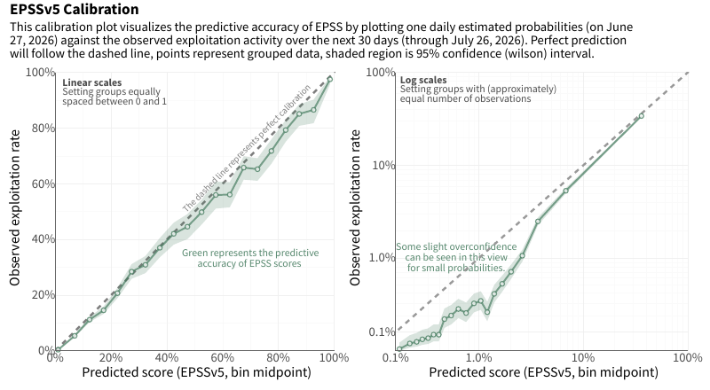
Why 30 days. The window is chosen (without much fanfare) to match practitioner decision cycles. Patch Tuesday has anchored vulnerability response cadence for decades, and most vulnerability management programs are built around it. A 30-day prediction window maps onto that cycle: the score answers whether this vulnerability is likely to be exploited before the next patch window closes.
Daily re-scoring. The production model is not retrained daily. Each day, EPSS recomputes features for every vulnerability in the corpus and runs the fixed model to generate updated scores. Scores change because the inputs change. A score that moves from 0.02 to 0.15 overnight means new signals arrived — exploit code became available, chatter spiked and so on. The model itself is unchanged.
Retraining. The production model is retrained when performance monitoring indicates drift from the calibrated baseline. The measures used to detect that drift and the evidence threshold that triggers a retrain are covered in the next section.
Any system that tells you which vulnerabilities to prioritize is making a claim about which ones will be exploited. Most never demonstrate that the claim is true. They do not provide a baseline. They do not share any outcome measurement. There is no way for a practitioner to know whether following the scores left them better or worse off than ignoring them. The field has largely treated measurement as optional, and practitioners have been asked to accept prioritization systems on good stories, anecdotes and faith rather than evidence. Organizations pay billions annually for scanning tools, patch platforms, and risk dashboards. The core question those tools exist to answer goes unmeasured: which vulnerabilities will actually be exploited
EPSS is built around a feedback loop: scores are published daily, and exploitation outcomes are observed independently. We make a claim about what will happen in the next 30 days. We wait 30 days while continually collecting what is happening and then we measure. That structure removes the need for anecdotes and stories, the evidence is in the measurement.
Why accuracy is the wrong measure. The most intuitive performance metric is accuracy and it measures the fraction of correct predictions. But in the world of vulnerability exploitation activity, it can be very misleading. The large majority of vulnerabilities are never exploited in any given 30-day window. A simple rule that predicts zero exploitation for everything achieves accuracy around 97-98%. The metric tells you nothing about whether the model is useful, because it rewards the prediction that requires no model at all. As a general rule of thumb, accuracy should not be the metric when there is an imbalance in the outcome data (in our case, exploitation activity).
EPSS uses three performance measurements: coverage, effort, and efficiency.
- Coverage is the fraction of exploited vulnerabilities a given score threshold captures. If EPSS flags 500 vulnerabilities and those 500 include 80% of the vulnerabilities that were actually exploited in the following 30 days, coverage is 80%. In statistical terms, coverage is recall.
- Effort is the fraction of all vulnerabilities you must act on to achieve a given level of coverage. Remediating 500 vulnerabilities out of a total population of 200,000 represents an effort of 0.25%.
- Efficiency is the fraction of vulnerabilities you acted on that were actually exploited. Of those 500 flagged vulnerabilities, if 100 were exploited, efficiency is 20%. High efficiency means a low proportion of remediation effort was spent on vulnerabilities that were never going to be exploited. In statistical terms, efficiency is precision. The terms coverage and efficiency deliberately replace recall and precision because they describe the practitioner's decision more directly than their statistical equivalents.
The coverage-efficiency curve. The first plot shows efficiency on the vertical axis and coverage on the horizontal axis, across the full range of possible EPSS score thresholds. Moving left along the curve represents a higher threshold with fewer vulnerabilities flagged, higher efficiency but lower coverage. Moving along the line from the top left to the bottom right, the cutoff threshold drops through the range, each step adds more vulnerabilities to be prioritized and creates higher coverage at a cost of lower efficiency. The tradeoff between coverage and efficiency at any given threshold is one of the primary considerations.
The plot includes two reference points. The random baseline shows the efficiency a random selection of vulnerabilities would achieve at each coverage level: as you randomly pull more vulnerabilities into scope, efficiency stays flat at the base exploitation rate regardless of how many you select. CVSS-based thresholds appear as specific points on the same axes, showing the coverage and efficiency achieved by remediating all vulnerabilities above a severity cutoff. The EPSS curve sits substantially above both at most coverage levels, meaning it achieves higher efficiency at equivalent coverage than either alternative.
The gain curve. The second plot shows coverage on the vertical axis and effort on the horizontal axis. Starting from the highest EPSS scores and working down, how quickly does coverage accumulate as effort increases?
The random baseline here is a diagonal: selecting vulnerabilities at random, coverage grows proportionally with effort. A prioritization method with no predictive value produces a curve that follows the diagonal. The EPSS curve rises steeply above the diagonal at low effort levels, meaning a small fraction of the vulnerability population captures a disproportionately large fraction of exploited vulnerabilities. The CVSS comparison again appears as a point: the coverage achieved by the CVSS-based population at the effort that population represents.
The two plots describe the same result from different angles. The coverage-efficiency curve answers: for a given level of coverage, how efficiently am I spending remediation effort? The gain curve answers: for a given level of effort, how much of the exploited population am I capturing? Both are useful depending on how a practitioner's constraints are framed.
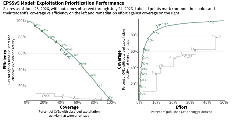
How performance is measured during tuning. The precision-recall and gain curves are the communication instrument we use to describe performance to practitioners. During model development and tuning, performance is tracked using the area under the precision-recall curve (PR-AUC) and log-loss, which measures how closely the model's probability estimates match observed outcomes. These aggregate statistics are less intuitive but more tractable when comparing many model configurations against each other during iterative development.
Ongoing monitoring. Scores published 30 days ago can be evaluated against the exploitation activity observed in the 30 days that followed. EPSS monitors this continuously. Daily fluctuation in the curves is expected. The trend over time is the signal: sustained drift toward the baselines indicates the model is losing predictive power as the threat landscape evolves. That trend is what triggers a retraining cycle.
Known limitations
Model limitations
Population-level scores. EPSS scores reflect exploitation probability across the entire observed population of known vulnerabilities. They are not tailored to any specific organization, industry, or technology stack. A vulnerability widely deployed in your environment without compensating controls may score low. A vulnerability actively exploited against a technology your organization does not run may score high. The score is an accurate population-level estimate; it is not a statement about any specific instance or exposure. Practitioners should layer EPSS scores with asset inventory and other local context to determine which high-scoring vulnerabilities are actually present in their environment.
Sparse signal on newly disclosed vulnerabilities. On the day a vulnerability is disclosed, the publicly available information may be thin. Chatter has not yet accumulated. Exploit code may not exist. No exploitation activity has been observed. EPSS still produces a score from that sparse record, and the score is accurate given the available signal, but the signal is limited. Scores for newly disclosed vulnerabilities should be interpreted with that constraint in mind. As signal accumulates over subsequent days and weeks, scores update to reflect it. This should not be interpreted to mean that all newly disclosed vulnerabilities score low, there are absolutely vulnerabilities that come out of the gate swinging (as one would say). This is just acknowledging that often times, and especially given the rising rate of published vulnerabilities, it may take some time for the public information to catch on that something is important and the data, as well as EPSS, reflects that.
Calibrated probability, not a binary classification. A score of 0.05 means a 5% probability of exploitation, or around 1 in every 20, within 30 days across the population. It should not be mistakenly taken as a declaration that the vulnerability is safe. Across a population of 10,000 scored vulnerabilities, a 5% score on every one of them corresponds to 500 exploitation events. Low scores cluster most vulnerabilities because exploitation at the population level is genuinely rare, not because those vulnerabilities carry no risk. The score should be read as a probability and used as a prioritization input, not as a pass/fail threshold.
Observation bias in training labels. EPSS trains on exploitation activity its data partners can observe. Exploitation that generates no endpoint telemetry, no IPS alert, no honeypot traffic, and no threat intelligence report does not appear in the training data. The model learns from a sample of actual exploitation, not a census of it. The scores reflect the threat landscape as seen through a specific set of sensors, not as it exists in totality.
Environmental limitations
Several conditions that practitioners attribute specifically to EPSS as limitations apply equally to every vulnerability prioritization approach. They are features of the problem, not the model.
Cold start is universal. When a vulnerability is disclosed, every practitioner faces the same sparse information environment that EPSS does. The practitioner without EPSS searches for blog posts, vendor advisories, and social media commentary, often chasing the same hot takes that circulate for days before any exploitation data exists. EPSS ingests those same sources alongside threat intelligence feeds, exploit repository data, and domain reference signals, weights them against historical patterns for similar vulnerabilities, and produces a calibrated estimate. The cold start problem does not disappear without EPSS; it is handled informally and inconsistently instead.
Observation gaps affect everyone. No intelligence source has complete visibility into exploitation activity. The manager who escalates a vulnerability because of a news article acts on a single data point from a single source with unknown reliability and unknown relevance to the organization's environment. EPSS aggregates nearly a dozen independent data sources of exploitation activity across four distinct sensor types, each with different coverage profiles and detection mechanisms. A gap in what EPSS can observe is most likely a gap in what anyone can observe. The difference is that EPSS makes its sources and methods explicit rather than leaving the practitioner to assess the reliability of each informal signal independently.
The limitations often attributed to EPSS are the conditions of the field. Incomplete information, newly disclosed vulnerabilities with uncertain risk, exploitation activity that is hard to observe and these are not EPSS-specific failures. They are the environment every vulnerability management program operates in. EPSS does not eliminate that environment but it is a more systematic response than the alternatives.
EPSS is maintained by the EPSS Special Interest Group at FIRST. Scores are generated by Empirical Security and published freely to the community.